Deep Neural Network and Gaussian Processes

A Gaussian Process is characterized by a collection of functions that map any \(\mathbf{x}\in \mathbb{R}^d\) to a Gaussian random variable \(f(\mathbf{x})\). We can use the notation \(F\) for the random object, and \(f\) any realisation. Hence, each function \(f\) can be associated with a probability \(\mathbb{P}(F=f)\). Working on the function space can be conceptually challenging, that's why it is way much easier work with the images \(f(\mathbf{x})\). 

In its simplest form, it has a zero mean \(\mathbb{E}[f(\mathbf{x})]\) for any \(\mathbf{x}\). Considering two input values \(\mathbf{x}\) and \(\mathbf{x'}\), the covariance between \(f(\mathbf{x})\) and \(f(\mathbf{x'})\) is given by the kernel function of the Gaussian Process:

$$Cov\left(f(\mathbf{x}),f(\mathbf{x'})) = K(\mathbf{x},\mathbf{x'}\right)$$

When considering a set of points \(\mathbf{X} = (x_1,x_2,\dots,x_n)^\top\), you will notice that the resulting image vector is in fact a Gaussian vector of covariance matrix \(K(\mathbf{X},\mathbf{X}) = \left[K(x_i,x_j)\right]_{1\leq i,j \leq n}\):

$$f(\mathbf{X}) = \begin{pmatrix} f(x_1)\\ f(x_2)\\ \vdots\\ f(x_n)\end{pmatrix} \sim \mathcal{N} \left( \mathbf{0},K(\mathbf{X},\mathbf{X})\right)$$

A Gaussian Process is a very interesting tool since it describes a phenomenon in space that is random but still has a structure that is given by the kernel function.

Relating the kernel function to the behaviour of \(f\)

Let's consider the most comon kernel function: the Radial Basis Function (RBF):

$$K_{\text{RBF}} (\mathbf{x},\mathbf{x'}) = \sigma^2 e^{-\frac{||\mathbf{x}-\mathbf{x'}||^2}{2\ell^2}}$$

One can notice that the covariance between \(f(\mathbf{x})\) and \(f(\mathbf{x'})\) increases as \(\mathbf{x}\) approaches \(\mathbf{x'}\). We expect any realisation of \(F\) to be continuous. More generally, the parameter \(\ell\) will determine how fast does any realisation \(f\) change for different \(x\).

Training a Gaussian Process on a dataset

A Gaussian Process can be used as a predictive model for regression by deriving the probability distribution of \(F\) after observing some values \((y_1,y_2,\dots,y_d)\) at the locations \((x_1,x_2,\dots,x_d)\). We assume that: \( y_i = f(x_i) + \epsilon_i \) with \( \epsilon_i \sim N(0, \sigma^2) \), which means our observation have a small white noise error. We use a zero-mean Gaussian Process (GP) as the prior distribution over \( f(\cdot) \): \( f(\cdot) \sim GP(0, k(\cdot, \cdot)) \). To generate predictions, we start by concatenating our training and test vectors:

$$\begin{aligned}\begin{pmatrix}Y \\ Y^*\end{pmatrix}&=\begin{pmatrix}f(X) \\ f(X^*)\end{pmatrix}+\begin{pmatrix}\epsilon \\ \epsilon^*\end{pmatrix} \\&=\mathcal{N}\left(0,\begin{pmatrix}k(X, X)+\sigma^2 I & k(X, X^*) \\k(X^*, X) & k(X^*, X^*)+\sigma^2 I\end{pmatrix}\right)\end{aligned}$$

Now, we simply need to condition \( Y^* \) on the other variables:

$$ P(Y^* \mid Y, X, X^*) \sim N(\mu, \boldsymbol{\Sigma}) $$

where:

$$\begin{aligned}\mu &= k(X^*)\left(k(X, X)+\sigma^2 I\right)^{-1} Y \\\boldsymbol{\Sigma} &= k(X^*, X^*)+\sigma^2 I - k(X^*, X)\left(k(X, X)+\sigma^2 I\right)^{-1} k(X, X^*)\end{aligned}$$

You can see that computing the posterior (with is equivalent to 'train' our models) requires a matrix inversion that is very computationally demanding for large dataset (\(O(n^3)\) for an \(n\times n \) matrix).

Gaussian Process (GP) VS Deep Neural Network (DNN)

\[\begin{array}{|l|c|c|}\hline\textbf{Name} & \textbf{Gaussian Processes (GP)} & \textbf{Deep Neural Networks (DNN)} \\\hline\textbf{Model Type} & \text{Non-parametric} & \text{Parametric} \\\hline\textbf{Operation} & \text{Bayesian, Probabilistic Inference} & \text{Via gradient and supervised learning} \\\hline\textbf{Assumptions} & \text{Assumptions on the function (smooth function, etc.)} & \text{No assumptions} \\\hline\textbf{Uncertainty} & \text{Quantification of uncertainty} & \text{No quantified uncertainty} \\\hline\textbf{Complexity} & \mathcal{O}(n^3) \text{ for matrix inversion} & \mathcal{O}(n) \text{ per optimization iteration} \\\hline\textbf{Capabilities} & \text{Capture of complex dependencies} & \text{Learning of complex relationships} \\\hline\textbf{Usage} & \text{Small datasets, uncertainty analysis} & \text{Large datasets} \\\hline\end{array}\]

DNNs can be trained on extremely large datasets. This is mainly possible thanks to backpropagation and gradient computation. However, for regression or classification tasks, it does not provide any indication of the model's confidence in its predictions.

On the other hand, GPs cannot be trained on very large datasets, as shown previously, but they provide a posterior probabilistic distribution that can be very valuable for inferences. You can find the main pros and cons of both methods in the following table:

Bayesian Deep Neural Network

A DNN can be seen as a function \(f_{\mathbf{w}}\) which is defined on the feature space and is parametrized by the vector \(\mathbf{w}\). The parameters are the weights of the neural network. An optimal weight vector \(\mathbf{w_*}\) if found by minimizing the loss function of our dataset and a regularization term. With this method, the function can now map any vector \(\mathbf{x}\) of the feature space to a prediction \(f_{\mathbf{w}}(\mathbf{x})\). However, we have now information about the confidence of our model. As a matter of fact, regions that are not well covered by our dataset have a higher uncertainty that is not reflected by our DNN. Let's consider another approach: the Bayesian Inference.

In the Bayesian inference, our weight vector is now considered as a distribution in the parameters space. Instead of describing the neural network parameters with a unique vector, we consider every possible parameters and would like to compute the probability of each of them with respect to our observations. Now for any vector \(\mathbf{x}\) of the feature space, we can derive the posterior distribution \(p\big(f_{\mathbf{w}}(\mathbf{x})\mid \mathcal{D}\big)\) which gives all the possible values given you observed data \(\mathcal{D}\) and how likely they are.

In practice, Deep Neural Networks have too many parameters to allow Bayesian Inference. The idea of [Khan et al., 2020] is to approximate a trained DNN with a GP that gives similar output. Combining a DNN and its GP is a way to approximate a Bayesian Inference Model of your DNN.

Construction of GP approximation

The goal of this process is to approximate the posterior distribution of weights in a deep neural network using a Gaussian Process, which can be more computationally efficient than traditional Bayesian inference methods.

Define the Joint Probability

The first step involves defining the joint probability of the weights \(\mathbf{w}\) and the data \(\mathcal{D}\):

\[p(\mathbf{w}, \mathcal{D}) = \prod_{i=1}^N p(\mathbf{x_i},\mathbf{y_i}\mid \mathbf{w})p(\mathbf{w})\]

This can be rewritten using the loss function \(\ell\) and a Gaussian prior on the weights:

\[p(\mathbf{w}, \mathcal{D}) = \prod_{i=1}^N e^{-\ell(y_i,\mathbf{f_w}(x_i))}p(\mathbf{w}) = e^{-\sum_{i=1}^N \ell(y_i,\mathbf{f_w}(x_i))+\frac{1}{2}\delta\mathbf{w}^\top\mathbf{w}}\]

Compute the Posterior Distribution

Next, we compute the posterior distribution of the weights given the data:

\[p(\mathbf{w}\mid \mathcal{D}) = \frac{p(\mathbf{w},\mathcal{D})}{p(\mathcal{D})} \propto e^{-\sum_{i=1}^N \ell(y_i,\mathbf{f_w}(x_i))+\frac{1}{2}\delta\mathbf{w}^\top\mathbf{w}}\]

Approximate the Posterior with a Gaussian Distribution

To simplify the posterior, we approximate it with a Gaussian distribution:

\[p(\mathbf{w} \mid \mathcal{D}) \approx \mathcal{N}(\mathbf{w} \mid \boldsymbol{\mu}, \boldsymbol{\Sigma})\]

This approximation is often referred to as Laplace's Approximation.

Visualize the Approximation

We visualize the approximation using a quadratic surface, which represents the negative log-posterior:

\[-log \left(p(\mathbf{w} \mid \mathcal{D})\right) \approx \frac{1}{2}(\mathbf{w}-\mathbf{w^*})^\top \mathbf{H} (\mathbf{w}-\mathbf{w^*}) \approx \frac{1}{2} (\mathbf{w}-\mathbf{\mu})^\top \mathbf{\Sigma}^{-1} (\mathbf{w}-\mathbf{\mu})\]

Compute the Precision Matrix

Finally, we compute the precision matrix \(\boldsymbol{\Sigma}^{-1}\), which is the second derivative of the negative log-posterior evaluated at the mode \(\mathbf{w_*}\):

\[\boldsymbol{\Sigma}^{-1} = \nabla_{w w}^{2} \left( -\sum_{i=1}^N \ell_i(\mathbf{w})(x_i))+\frac{1}{2}\delta\mathbf{w}^\top\mathbf{w}\right)(\mathbf{w_*}) = \sum_{i=1}^{N} \nabla_{w w}^{2} \ell_{i}\left(\mathbf{w}_{*}\right)+\delta \mathbf{I}_{P}\]. The previous steps allowed us to create a model that approximates the posterior distribution of our DNN. In the following section, this model will be referred to as the DNN-Laplace model.

An interesting property is highlighted by [Dutordoir et al., 2020], where a Deep Neural Network with infinitely large layers will converge to a Deep Gaussian Process. This—to avoid delving into the details—corresponds more or less to a concatenation of several Gaussian Processes.

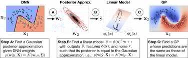
Find a Linear Model that approaches the posterior

Once the \(\mathbf{w}\) posterior distribution has been approximated, the idea of [Khan et al., 2020] is to find a linear model \(\tilde{y} = \phi(\mathbf{x})^\top\mathbf{w} + \epsilon\). This model is in fact the desired model. The construction of \( \phi(\mathbf{x})\) is complicated and will not be discussed here. This additional step approximates the DNN-Laplace model with a Gaussian Process. The resulting approach will be referred to as DNN2GP-Laplace.

Testing DNN2GP on datasets

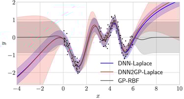
Regression Task

Let's first try the model on a regression task based on [Snelson et Ghahramani, 2005] dataset. The behavior of the DNN2GP-Laplace posterior distribution is compared with the one obtained from a RBF Gaussian Process (RBF-GP). As a reminder, this experiment aims to compare DNN2GP-Laplace with a GP on a simple dataset where both models can be trained. On more complicated dataset, GP training is untractable as explained previously.

The DNN-Laplace model corresponds to the approximation of the posterior distribution of the Deep Neural Network.

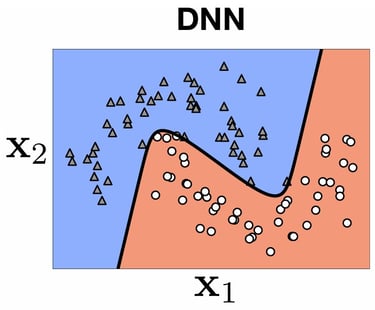
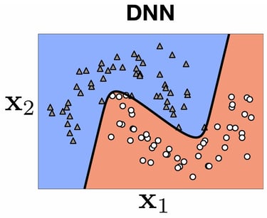
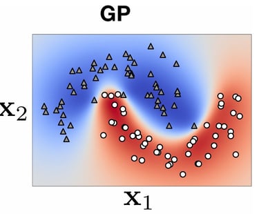
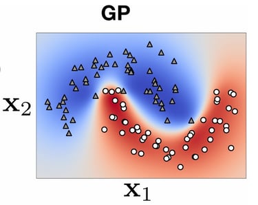
Classification tasks

In this section, we present the results of different models on classification tasks using MNIST and CIFAR-10 datasets.

MNIST, with its well-defined structure of handwritten digits, shows strong intra-class correlations in the kernel matrix, resulting in high test accuracy. In contrast, CIFAR-10, with its more complex natural images, presents a noisier kernel matrix, indicating greater difficulty in learning and lower test accuracy. This suggests that DNN2GP captures the structure well on simpler datasets but faces more uncertainty with complex ones.

Visualizing the kernel matrices for MNIST and CIFAR-10 further supports these findings. The analysis of uncertainties on CIFAR-10 reveals low epistemic uncertainty, indicating model confidence, but high aleatoric uncertainty, suggesting noise in the labels. The model's lack of flexibility contributes to the difficulty in separating classes.

Optimizing hyperparameters, such as δ, using the GP marginal likelihood is another key aspect. This approach avoids the need for cross-validation and helps prevent underfitting and overfitting by identifying the optimal δ. It serves as an efficient alternative for tuning DNN hyperparameters.

On this graph, on can see that the GP-RBF model tends to assume zero-mean valued distribution far form observed points. This comes from the facts that the model returns the prior distribution when at locations where no data have been observed. The DNN-Laplace model on the other hand extrapolates the behaviour of the closest data cluster. However, it seems to be overconfident on its prediction. Finally, DNN2GP-Laplace gives a similar result, but the posterior distribution's standart deviations grows significantly faster as one strays from observed regions.

Figure from [Khan et al.,2020]

Figure from [Khan et al.,2020]

Figures from [Khan et al.,2020]

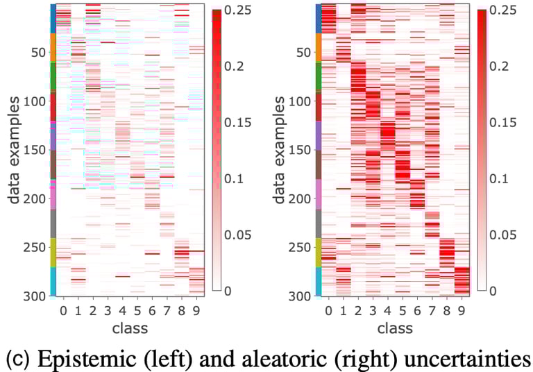
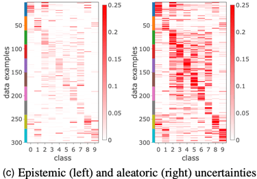
Figure from [Khan et al.,2020]

Bibliography

Dutordoir, Vincent, James Hensman, Mark van der Wilk, Carl Henrik Ek, Zoubin Ghahramani, et Nicolas Durrande. 2021. « Deep Neural Networks as Point Estimates for Deep Gaussian Processes ». arXiv. https://doi.org/10.48550/arXiv.2105.04504.

Khan, Mohammad Emtiyaz, Alexander Immer, Ehsan Abedi, et Maciej Korzepa. 2020. « Approximate Inference Turns Deep Networks into Gaussian Processes ». arXiv. https://doi.org/10.48550/arXiv.1906.01930.

Snelson, Edward, et Zoubin Ghahramani. 2005. « Sparse Gaussian Processes using Pseudo-inputs ». In Advances in Neural Information Processing Systems. Vol. 18. MIT Press. https://papers.nips.cc/paper_files/paper/2005/hash/4491777b1aa8b5b32c2e8666dbe1a495-Abstract.html.